Probability Series - Part-2 - Discrete Random Variable
A tutorial on basic concepts related to Probability.


- Note
- Introduction
- Discrete Random Variable
- Probability Mass Function
- Probability Distribution Function (Cumulative distribution function)
- Properties of Probability Distribution Function
- Examples of Discrete Random Variables
- Real Life Use Cases of These Distributions
- References
Introduction
This is the second part of our Probability Series where we will talk about Random Variables.Before we start with random variable lets take a look at some of the concepts we discussed in the previous post:
The world we see around us is full of phenomena we perceive as random or unpredictable. We aim to model this phenomena as outcomes of some experiment. The outcomes are a result of sample space and subsets of sample space are called events. The events will be assigned a probability a number between 0 and 1 that expresses how likely the event is to occur.
The sample space associated with an experiment, together with a probability function defined on all its events, is a complete probabilistic description of that experiment. Often we are interested only in certain features of this description. We focus on these features using random variables.
Random Variables can be expressed in two forms:
- Discrete Random Variable
- Continuos Random Variable
Discrete Random Variable
Suppose we are playing a game where the moves are determined by the maximum of two independent throws with a die. So here our sample space (Ω) is $ [(w_1,w_2) : w_1,w_2 \in {1,2,3..6}]$ = $[(1,1)(1,2)..(1,6),(2,1)...(6,6)]$. So our sample space is of size 36.
The events we are interested in is when we throw dice twice ,we will take the maximum of two independent throws.So for example if in one throw we get 2 and in another 3 , we will consider the outcome of this event as 3.
Let us represent this function as $S$ which describes what an outcome could be for an event using the following:
$S(w_1,w_2) = max(w_1,w_2)$ for $w_1,w_2 \in Ω$
Then the values S can take will be between 1 and 6 i.e $S \in [1,2,3..6]$
The functions S here is an examples of what we call discrete random variables.
Let us now look at the formal defintion and try to relate with our example :
Discrete Random Variabe
Let Ω be a sample space. A discrete random variable is a function X : Ω → R that takes on a finite number of values $a_1 , a_2 , . . . , a_n$ or an infinite number of values a_1 , a_2 , . . . .
In a way, a discrete random variable X transforms a sample space Ω to a more tangible sample space Ω̃, whose events are more directly related to what we are interested in.If we link this to our example the thing we were interested in was the outcome as a $max(w_1,w_2)$ and the function describing this $S$ is precisely what we are calling as Discrete Random Variable which can take values $\in[1,2,3,4,5,6]$
Probability Mass Function
Continuing with our earlier example, as we have now introduced $S$ as a our Discrete Random Variable ,which represents a newer sample space Ω̃, hence the sample space Ω is no longer important. It suffices to list the possible values of $S$ and their corresponding probabilities.The particular function in which this information is contained about $S$ is called Probability Mass function of $S$
Definition
The probability mass function p of a discrete random variable X is the function p : R → [0, 1], defined by:
p(a) = P(X = a) for $− ∞ < a < ∞$
If X is a discrete random variable that takes on the values $a_1 , a_2 , . . .$, then:
- $p(a_i ) > 0,$
- $p(a_1 ) + p(a_2 ) + · · · = 1,$
- $p(a) = 0$ for all other a.
If we link it to our example now:
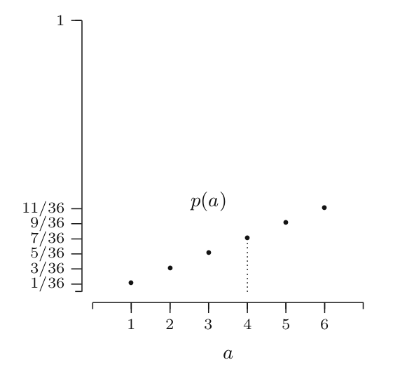
Probability mass function p of $S$ for different values of a will be:
$p(a=1) = 1/36$ when $w_1,w_2 \in [(1,1)]$
$p(a=2) = 3/36$ when $w_1,w_2 \in [(1,2),(2,1),(2,2)]$
$p(a=3) = 5/36$ when $w_1,w_2 \in [(1,3),(2,3),(3,1),(3,2),(3,3)]$
.....
$p(a=6) = 11/36$
and p(a) = 0 for all other values of a
Probability Distribution Function (Cumulative distribution function)
Definition
The distribution function F of a random variable X is the function F : R → [0, 1], defined by F (a) = P(X ≤ a) for −∞ < a < ∞
The distribution function F of a discrete random variable X can be expressed in terms of the probability mass function p of X and vice versa as both the probability mass function and the distribution function of a discrete random variable X contain all the probabilistic information of X.
So if we have to calculate the PDF of our previously define discrete random variable X which can take values $a_1,a_2,a_3...$ where PMF was defined as $p(a_i), p(a_2 ), p(a_3 )...$
$$F(a) = \sum\limits_{a_i<=a} p(a_i)$$
 We see that, for a discrete random variable X, the distribution function F jumps in each of the $a_i$ , and is constant between successive $a_i$ . The height of the jump at $a_i$ is $p(a_i )$, in this way p can be retrieved from F.
Properties of Probability Distribution Function
Based on our understanding on Probablity Distribution function, we can now define some properties that will help us to identify any function as distribution function of some random variable. These properties are as follows:
- For $a ≤ b$ one has that $F(a) ≤ F(b).$ This property is an immediate consequence of the fact that $a ≤ b$ implies that the event $\{X ≤ a\}$ is contained in the event $\{X ≤ b\}$.
- Since $F(a)$ is a probability, the value of the distribution function is always between 0 and 1. Moreover,
$$\lim_{a \to +\infty} F(a) = \lim_{a \to +\infty} P(X ≤ a) = 1$$ $$\lim_{a \to -\infty} F(a) = \lim_{a \to -\infty} P(X ≤ a) = 0$$
- F is right-continuous, i.e. $$\lim_{\epsilon \to 0} F(a + \epsilon) = F(a)$$
Examples of Discrete Random Variables
Bernoulli Distribution
The Bernoulli distribution is used to model an experiment with only two possible outcomes, often referred to as “success” and “failure”, usually encoded as 1 and 0.
A discrete random variable X has a Bernoulli distribution with parameter p, where $0 ≤ p ≤ 1$, if its probability mass function is given by
$Ber(p)$
$$p_x(1) = P(X = 1) = p$$
$$and$$
$$p_X(0) = P(X = 0) = 1 − p$$
Let us take an example of a coin toss.We say X=1 means getting Head and X = 0 means getting tails.Now if the coin is unbiased then P(X=1) = P(X=0) = p = 0.5. But if we say the coin is biased towards heads with 0.9 then P(X=1) = 0.9 and P(X=0) = 0.1. And now if generalize this for any value of biasness say $p→[0,1]$ we can say :
$$P(X=1/p) = p$$
$$P(X=0/p) = 1-p$$
or in general
$$P(X|p) = p^x.(1-p)^{1-x}$$
Here we have introduced a parameter p which is unknown and the objective of learning is to observe bunch of 1s and 0s and figure out p. We will talk about the parameter p in our further sections.
Expectation/Mean of Bernoulli Variable
$$E(X|p) = \sum\limits_{x \epsilon [0,1]} x.p(x|p)$$$$= 1.P(X=1|p) + 0.P(X=0|p)$$
$$= 1.P(X=1|p)$$
$$= p$$
So for Bernoulli Distribution the Expectation is the same as the Probability
Variance of Bernoulli Variable
$$Var(X|p) = E[(X-E(X|p)^2|p]$$
$$= E[(X-p)^2|p]$$
$$=(1-p)^2.P(X=1|p) + (0-p)^2.P(X=0|p)$$
$$=(1-p)^2.p + p^2 . (1-p)$$
$$=p.(1-p)$$
Binomial Distribution
A binomial distribution can be thought of as simply the probability of getting HEAD or TAIL outcome in an experiment or survey that is repeated multiple times.The other way to see this is that the Bernoulli distribution is the Binomial distribution with n=1.
Definition A discrete random variable X has a binomial distribution with parameters n and p, where n = 1, 2, . . . and 0 ≤ p ≤ 1,if its probability mass function is given by
$$Bin(n, p)= p_x(k) = P(X = k) = (n|k)p^k(1-p)^{n-k}$$
Here,
- The first variable in the binomial formula, n, stands for the number of times the experiment runs.
- The second variable, p, represents the probability of one specific outcome.
Let's take an example to get the hang of this concept: Consider the game of coining the toss. It consists of 10 trials, and each trial has equal probability of getting heads and tails. You will win the game if you get exactly 1 head in those 10 trials.What is the probability that you will win the game P(W) = ?
$n= 10$, $p = 1|2$
Out of 10 trials ,we can get head in any one of 10 trials.So there are 10 ways in which this can happen and if you remember thisfrom Permutation and Combination concepts we can represent this as $10C_1$.Also it means we have to get tails 9 times and heads 1 time to win the game.Hence
$$P(W) = 10C_1. (1/2)^1(1/2)^{10-1}$$
Now let us modify the experiment setting by saying that the coin is biased where $P(Head) = 1/4$ and $P(Tails) = 3/4$. What is the probability that you will win the game P(X),given winning is defined by getting 6 heads and more out of 10 trials.
Possible cases of winning could be:
- Getting 6 heads and 4 tails
- Getting 7 heads and 3 tails
- Getting 8 heads and 2 tails
- Getting 9 heads and 1 tails
- Getting all 10 heads So, $$P(X ≥ 6) = P(X = 6) + · · · + P(X = 10)$$
$$P(X≥6) = 10C_6 . (1/4)^6(1/4)^{10-6} + 10C_7 . (1/4)^7(1/4)^{10-7 }... + 10C_10 . (1/4)^10(1/4)^{10-10}$$ $$P(X ≥ 6) = 0.0197$$
The preceding random variable W or X are examples of a random variable with a binomial distribution with parameters n = 10 and p = 1/2
Expectation/Mean of Binomial Distribution
If we carefully think about a binomial distribution, it is not difficult to determine that the expected value of this type of probability distribution is np. For a few quick examples of this, consider the following:
- If we toss 100 coins, and X is the number of heads, the expected value of X is 50 = $(1/2)*100.$
Although intuition is a good tool to guide us, it is not enough to form a mathematical argument and to prove that something is true.Lets try calculating it..
The probability function for a binomial random variable is: $$b(x;n,p) = (n|x)p^x(1-p)^{n-x}$$ This is the probability of having $x$ successes in a series of $n$ independent trials when the probability of success in any one of the trials is $p$. If $X$ is a random variable with this probability distribution,then Expectation:
$$E(X) = \sum\limits_{x = 0}^{n} x.(n|x).p^x.(1-p)^{n-x}$$or
$$E(X) = \sum\limits_{x = 0}^{n} x.[n!|((x!)(n-x)!))].p^x.(1-p)^{n-x}$$Since each term of the summation is multiplied by x, the value of the term corresponding to x = 0 will be 0, and so we can actually write
$$E(X) = \sum\limits_{x = 1}^{n} [n!|(((x-1)!)(n-x)!))].p^x.(1-p)^{n-x}$$Now, Let y = x−1 and m=n−1. Subbing x=y+1 and n=m+1 into the last sum (and using the fact that the limits x= 1 and x=n correspond to y= 0 and y=n−1 = m, respectively
$$E(X) = \sum\limits_{y = 0}^{m} [(m+1)!|((y!)(m-y)!))].p^{y+1}.(1-p)^{m-y}$$We factor out the m+1 and one p from the above expression
$$E(X) = (m+1).p \sum\limits_{y = 0}^{m} [m!|((y!)(m-y)!))].p^{y}.(1-p)^{m-y}$$
Substituting m+1 = n
$$E(X) = n.p \sum\limits_{y = 0}^{m} [m!|((y!)(m-y)!))].p^{y}.(1-p)^{m-y} ----(i)$$
The binomial theorem says that
$$(a+b)^m =\sum\limits_{y=0}^{m} [m!|(y!)(m-y)!].a^y.b^{m-y}$$
Substituting a = p and b = 1-p in the above equation
$$E(X) = \sum\limits_{y = 0}^{m} [m!|((y!)(m-y)!))].p^{y}.(1-p)^{m-y}$$
and this is same as eq-1 if we ignore the $[n.p]$ part.Hence
$$(a+b)^m = (p+1-p)^m = 1$$
$$E(X) = np$$Similarly, if we put $y=x−2$ and $m=n−2$ we can get the Variance of Binomial Distribution.Try it yourself.You can also refer the materials which has been shared in the reference**
There is a more simpler way you can think about for calculating the Expectation and Variance of Binomial Distribution. Remember we said, Binomial Distribution is Bernoulli Distribution with n = 1.So extending on this concept we can say:
$$E(X) = I_1 + I_2 + I_3 ... I_n$$
where each I is the Independent Bernoulli Random Variable
We know Expecatation of Bernoulli Random Variable is p. So expectation for Binomial Distribution:
$$E(X) = E[I_1 + I_2 + I_3 + ....I_N]$$
$$E(X) = E[I_1] + E[I_2] + E[I_3] + .... E[I_N]$$
$$E(X) = p + p + p + p .. = np$$
On the same line ff we think about the Variance
$$Var(X) = Var[I_1 + I_2 + I_3 + ..I_N)$$
$$Var(X) = Var[I_1] + Var[I_2] + Var[I_3] + .... Var[I_N]$$
$$Var(X) = p(n-p) + p(n-p) .... = n. p(n-p)$$
Geometric Distribution
The geometric distribution is the distribution of the number of trials needed to get the first success in repeated Bernoulli trials.
Lets contiue on our previous example of coin toss to understand this concept:
Consider the game of coining the toss. It consists of 10 trials, and each trial has equal probability of getting heads and tails. You will win the game if you get exactly the 1st head in the 6th trial.What is the probability that you will win the game P(W) = ?
- P(H/T) = 0.5 ( as it mis mentioned we have equal probability og getting heads and tails).
- For the 1st Head to appear on the 6th trial:
- The first 5 trials must be a failure.
- The 6th trial must be a success.
Hence , if we calculate the P(W) at 6th trial:
$$P(W = 6) = 0.5^{(6-1)} * 0.5^1$$
$$P(W = 6) = 0.015625 ---- (i)$$
Now if we generalise :
Definition
A discrete random variable X has a geometric distribution with parameter p, where 0 < p ≤ 1, if its probability mass function is given by :
$$ p_x(k) = P(X = k) = (1 − p)^{k−1} * p$$where k = 1, 2, . . . .infinite steps (there is no upper bound on k)
Similarly if we ask:
Consider the game of coining the toss. It consists of 10 trials, and each trial has equal probability of getting heads and tails. You will win the game if the 1st head occurs on or before the third trial.What is the probability that you will win the game P(W) = ?
Ans
In short what we are looking for is : $P(X \leq 3)$
So
$$P(X \leq 3) = P(X=1) + P (X=2) + P(X=3)$$
$$P(X \leq 3) = (1-0.5)^0 * 0.5 + (1-0.5)^1 * 0.5 + (1-0.5)^2 * 0.5$$$$P(X \leq 3) = 0.5 + 0.25 + 0.125$$
$$P(X \leq 3) = 0.875 --- (ii)$$
or ,other way to think about this is to calculate $P(X>3)$ which means getting three failures(getting tails) in a row, then
$P(X\leq 3)$ is the compliemnt of $P(X>3)$, hence
$$P(X \leq 3) = 1 - P(X>3)$$
$$P(X \leq 3) = 1 - 0.5^3$$
$$P(X \leq 3) = 1 - 0.5^3$$
$$P(X \leq 3) = 0.875$$
This value is same as obtained in equation- (ii) above
#collapse
np.random.seed(123)
flips_till_heads = stats.geom.rvs(size=10000,  # Generate geometric data
                                  p=0.5)       # With success prob 0.5

# Print table of counts
print( pd.crosstab(index="counts", columns= flips_till_heads))

# Plot histogram
pd.DataFrame(flips_till_heads,columns=["Histogram of Geom Random Variable X"]).hist(range=(-0.5,max(flips_till_heads)+0.5)
                                    , bins=max(flips_till_heads)+1)
plt.ylabel("Frequency");

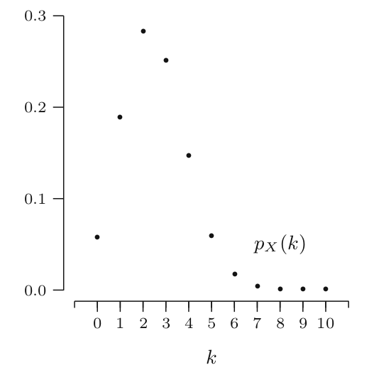
The distribution looks similar to what we'd expect: it is very likely to get a heads in 1 or 2 flips, while it is very unlikely for it to take more than 5 flips to get a heads. In the 10,000 trails we generated, the longest it took to get a heads was 12 flips.
#collapse
#If we calculate the mean of the distribution from our simulation:
flips_till_heads.mean()
We can observe this simulated value is very close to our theoretically calculated value.
Note-To get more precise value try increasing the number of trials,it will bring the mean closer to 2
#collapse
#If we calculate the mean of the distribution from our simulation:
flips_till_heads.var()
#collapse
p=0.5
fig, ax = plt.subplots(1, 1)
x = np.arange(stats.geom.ppf(0.01, p),

              stats.geom.ppf(0.99, p))

ax.plot(x, stats.geom.pmf(x, p), 'bo', ms=8, label='Geometric PMF')

ax.vlines(x, 0, stats.geom.pmf(x, p), colors='b', lw=5, alpha=0.5)
plt.title("Probability Mass Function")
plt.xlabel("X")
plt.ylabel("P(X)")

ax.legend(loc='best', frameon=False)

plt.show()

#collapse
#check the probability of seeing a specific number of flips before a successes
stats.geom.pmf(k=6,   # Prob of needing exactly 6 flips to get first success
              p=0.5)
This result is same as we obtained in equation (i) above
#collapse
p=0.5
fig, ax = plt.subplots(1, 1)
x = np.arange(1,max(flips_till_heads)+1)
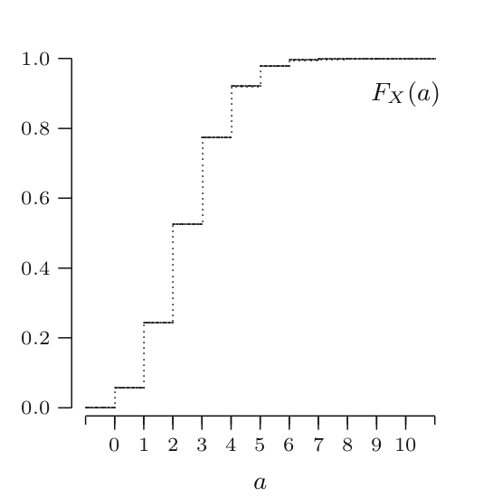
ax.plot(x, stats.geom.cdf(x, p), 'bo', ms=8, label='Geom CDF')
ax.vlines(x, 0, stats.geom.cdf(x, p), colors='b', lw=5, alpha=0.5)
ax.legend(loc='best', frameon=False)
plt.title("Probability Distribution Function")
plt.xlabel("X")
plt.ylabel("P(X)")
plt.show()

#collapse
#check the probability of needing 3 flips to get a success

first_three = stats.geom.cdf(k=3,   # Prob of success in first 3 flips
                           p=0.5)

first_three
This result is same as we obtained in equation (ii) above
#collapse
#To get more statistics of Geomtric distribution
p = 0.5
mean , var, skew, kurtosis = stats.geom.stats(p,moments = 'mvsk')
print(f'\n Mean- {mean}\n Variance- {var} \n Skewness- {skew} \n Kurtosis- {kurtosis}')
Real Life Use Cases of These Distributions
1. Bernoulli Distribution
Bernoulli distribution can model the following real life situations:
- A newborn child is either male or female. (Here the probability of a child being a male is roughly 0.5.)
- You either pass or fail an exam.
- A tennis player either wins or loses a match.
2. Binomial distribution
As we know Binomial distribution can be thought as Bernoulli with multiple trials in an experiment.
Binomial distribution can model the following real life situations:
- In an experiment of 100 pregnancy,finding the probability of number of child born is either male or female.
- In an experiment of test series,finding the probability of a students passing or failing an the test series.
- In a tennis tournament,finding the probability of a tennis player winning the tournament.
3. Geometric Distribution
Geometric distribution can model the following real life situations:
- In sports, particularly in baseball, a geometric distribution is useful in analyzing the probability a batter earns a hit before he receives three strikes; here, the goal is to reach a success within 3 trials.
- In cost-benefit analyses, such as a company deciding whether to fund research trials that, if successful, will earn the company some estimated profit, the goal is to reach a success before the cost outweighs the potential gain.
- In time management, the goal is to complete a task before some set amount of time.