Machine Learning Basics
A tutorial on basic concepts related to Machine Learning.
- Learning Algorithm
- Bias and Variance
- Underfitting and Overfitting
- Hyperparametes and Validation Sets
- Gradient Descent
- Example
A machine learning algorithm is an algorithm that is able to learn from data. But what do we mean by learning
The Task T
Machine learning tasks are usually described in terms of how the machine learning system should process an example.Many kinds of tasks can be solved with machine learning. Some of the most common machine learning tasks include the following:
- Classification
- Classification with Missing Inputs
- Regression
- Transcription
- Machine Translation
- Structured Output
- Anomaly Detection
- Synthesis and sampling
- Imputation of Missing Value
- Denoising
- Density Estimation or Probability Mass Function Estimation etc.
The Performance Measure, P
A quantitative measure to evaluate the abilities of a machine learning algorithm.Usually this performance measure P is specific to the task T being carried out.Some of the common measure includes the following:
- Accuracy
- Precision
- Recall
- ROC Curve
- F-score etc.
The Experience, E
Machine learning algorithms can be broadly categorized as unsupervised or supervised by what kind of experience they are allowed to have during the learning process.
- Supervised learning algorithms: Experience a dataset containing features,but each example is also associated with a label or target.
- Unsupervised learning algorithms: Experience a dataset containing many features, then learn useful properties of the structure of this dataset
- Reinforcement learning algorithms: Do not just experience a fixed Dataset but also revolves around States,Actions,Environment and Reward
In supervised machine learning an algorithm learns a model from training data.
The goal of any supervised machine learning algorithm is to best estimate the mapping function (f) for the output variable (Y) given the input data (X). The mapping function is often called the target function because it is the function that a given supervised machine learning algorithm aims to approximate.
$Y[pred] = f(x)$
$Y[true]= Y[pred] + Error (e)$
The prediction error for any machine learning algorithm can be broken down into three parts:
- Bias Error
- Variance Error
- Irreducible Error
The irreducible error cannot be reduced regardless of what algorithm is used. It is the error introduced from the chosen framing of the problem and may be caused by factors like unknown variables that influence the mapping of the input variables to the output variable.
Bias Error
Bias are the simplifying assumptions made by a model to make the target function easier to learn.
Generally, parametric algorithms have a high bias making them fast to learn and easier to understand but generally less flexible. In turn, they have lower predictive performance on complex problems that fail to meet the simplifying assumptions of the algorithms bias.
Low Bias: Suggests less assumptions about the form of the target function. High-Bias: Suggests more assumptions about the form of the target function. Examples of low-bias machine learning algorithms include: Decision Trees, k-Nearest Neighbors and Support Vector Machines.
Examples of high-bias machine learning algorithms include: Linear Regression, Linear Discriminant Analysis and Logistic Regression.
Variance Error
Variance is the amount that the estimate of the target function will change if different training data was used.
The target function is estimated from the training data by a machine learning algorithm, so we should expect the algorithm to have some variance. Ideally, it should not change too much from one training dataset to the next, meaning that the algorithm is good at picking out the hidden underlying mapping between the inputs and the output variables.
Machine learning algorithms that have a high variance are strongly influenced by the specifics of the training data. This means that the specifics of the training have influences the number and types of parameters used to characterize the mapping function.
Low Variance: Suggests small changes to the estimate of the target function with changes to the training dataset.
High Variance: Suggests large changes to the estimate of the target function with changes to the training dataset.
Generally, nonparametric machine learning algorithms that have a lot of flexibility have a high variance. For example, decision trees have a high variance
Examples of low-variance machine learning algorithms include: Linear Regression, Linear Discriminant Analysis and Logistic Regression.
Examples of high-variance machine learning algorithms include: Decision Trees, k-Nearest Neighbors and Support Vector Machines.

The goal of any supervised machine learning algorithm is to achieve low bias and low variance. In turn the algorithm should achieve good prediction performance.
As seen above
Parametric or linear machine learning algorithms often have a high bias but a low variance.
Non-parametric or non-linear machine learning algorithms often have a low bias but a high variance.
The parameterization of machine learning algorithms is often a battle to balance out bias and variance.

When training a machine learning model, we have access to a training set, we can compute some error measure on the training set called the training error, and we try to reduce this training error.
However our goal is not only to achieve minimum training error but also to make generalization error or the test error to be as low as possible
The factors determining how well a machine learning algorithm will perform are its ability to:
- Make the training error small.
- Make the gap between training and test error small.
The above two factors correspond to the two central challenges in machine learning:
Underfitting and Overfitting .
Underfitting occurs when the model is not able to obtain a sufficiently low error value on the training set.
Overfitting occurs when the gap between the training error and test error is too large.


Capacity
A model’s capacity is its ability to fit a wide variety of functions. Models with low capacity may struggle to fit the training set. Models with high capacity can overfit by memorizing properties of the training set that do not serve them well on the test set
We can control whether a model is more likely to overfit or underfit by altering its capacity
One way to control the capacity of a learning algorithm is by choosing its hypothesis space, the set of functions that the learning algorithm is allowed to select as being the solution. For example,in the above figure the linear regression algorithm has the set of all linear functions of its input as its hypothesis space. We can generalize linear regression to include polynomials, rather than just linear functions, in its hypothesis space. Doing so increases the model’s capacity.
Most machine learning algorithms have several settings that we can use to control the behavior of the learning algorithm. These settings are called hyperparameters. The values of hyperparameters are not adapted by the learning algorithm itself rather it is a trial and error method done iteratively.
But the question is on which data this model settings aka Hyperparameters needs to be learnt?
What is the problem if hyperparameters are learnt on training data?
If learned on the training set, such hyperparameters would always choose the maximum possible model capacity, resulting in overfitting.
To solve this problem, we need a validation set of examples that the training algorithm does not observe which guide the selection of hyperparameters.
Way to go
- Construct the validation set from the training data.
- Specifically,split the training data into two disjoint subsets.
- One of these subsets is used to learn the parameters.
- The other subset is our validation set, used to estimate the generalization error during or after training, allowing for the hyperparameters to be updated accordingly.
Generally we split the data as 70% train 30% valid or 80% train and 20% valid
But what if Data size is too small ??
Cross Validation
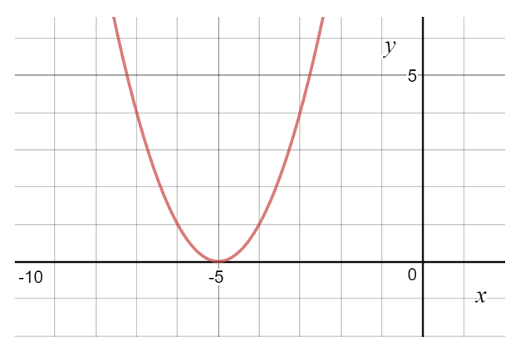
It is an optimization algorithm to find the minimum of a function. We start with a random point on the function and move in the negative direction of the gradient of the function to reach the local/global minima.
Nearly all of deep learning is powered by this very important algorithm with some twist :SGD:

The derivative $f'(x)$ gives the slope of $f(x)$ at the point x.In other words, it specifies how to scale
a small change in the input in order to obtain the corresponding change in the output.
The derivative is therefore useful for minimizing a function because it tells us how to change x in order to make a small improvement in y.We can thus reduce $f(x)$ by moving x in small steps with opposite sign of the derivative.
This technique is called gradient descent
When $f'(x) = 0$, the derivative provides no information about which direction to move. Points where $f'(x) = 0$ are known as critical points or stationary points
Types of Critical Points:
-
Local Minimum-Point where $f(x)$ is lower than at all neighboring points, so it is no longer possible to decrease $f(x)$ by making infinitesimal steps.
- Local Maximum Point where $f(x)$ is higher than at all neighboring points,so it is not possible to increase $f(x)$ by making infinitesimal steps.
- Saddle Points-Some critical points are neither maxima nor minima.
- Global Minimum-Point that obtains the absolute lowest value of $f(x)$

The gradient points directly uphill, and the negative gradient points directly downhill. We can decrease function $f$ by moving in the direction of the negative gradient. This is known as the method of steepest descent or gradient descent.
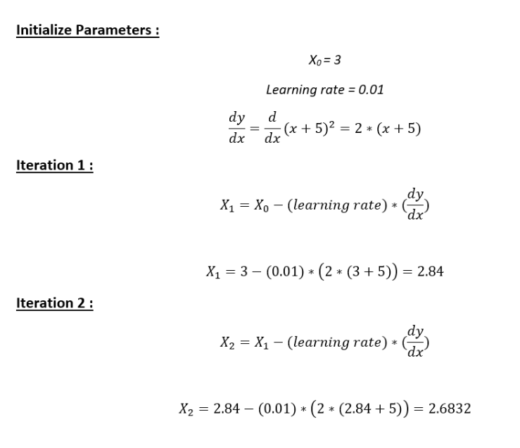
Now, let’s see how to obtain the same numerically using gradient descent.
#collapse
cur_x = 3 # Tell the algorithm from which point to start.Here we are saying the algorithm to start at x=3
rate = 0.01 # SIze of the step when we move in the direction of the steepest descent (Learning rate)
precision = 0.000001 #This tells us when to stop the algorithm
previous_step_size = 1 #
max_iters = 10000 # maximum number of iterations
iters = 0 #iteration counter
df = lambda x: 2*(x+5) #Gradient of our function
#collapse
while previous_step_size > precision and iters < max_iters:
    prev_x = cur_x #Store current x value in prev_x
    cur_x = cur_x - rate * df(prev_x) #Grad descent
    previous_step_size = abs(cur_x - prev_x) #Change in x
    iters = iters+1 #iteration count
    print("Iteration",iters,"\nX value is",cur_x) #Print iterations

print("The local minimum occurs at", cur_x)

